PREFACEThe main objective of this report is to suggest instruments for EMBLA 2000, and present general radioastronomy techniques, introduced to us by IRA. EMBLA 2000 has its origin in Erling Strand's research interest in the light phenomena in Hessdalen. As assistant professors at Hiø-IR, Erling Strand and Bjørn Gitle Hauge formed collaboration with the radioastronomy institute IRA to find an adequate way to investigate the light phenomena. We have performed the preliminary study for EMBLA 2000 at IRA in Medicina, Italy, in the period from 19th April to 28th May 1999. The institutions that supported our stay in Italy were the Norwegian State Education Loan Fund (flight expenses and food costs), the legacy of Halden Council, Hiø-IR, Servicesenteret as (Sarpsborg) and Alcatel Telecom, div. Telettra as. Angela Dennington has made it possible for us to present our report in English. We give her our warmest thanks. Any errors of any sort in the text, figures and data are our responsibility. We are very grateful to our supervisors Dr. Stelio Montebugnoli, Jader Monari and Sergio Mariotti at IRA and Bjørn Gitle Hauge at Hiø-IR for helping us with the project in all their capable ways. We would also like to express our deepest thanks to the staff at IRA for their excellent hospitality, and generous will to share their knowledge. They have made our stay in Italy an unforgettable experience.
EMBLA 2000
Sarpsborg - Medicina
SUMMARYDESCRIPTION OF THE GROUP
Our group consists of Petter Norli and Cecilie T. Langvik, and we are final year students at the School of Engineering and Natural Sciences (Hiø-IR), Østfold College. We both like to travel and meet other cultures, so we wanted to do our final year project abroad. The Department of Electronics and Telecommunications Engineering was in the process of establishing a collaboration project, EMBLA 2000, with Istituto di Radioastronomia in Bologna, Italy. As a consequence, we were given the fortunate opportunity of doing our project at the institute in Italy. Cecilie Terese Langvik is 21 years of age, and lives in her beloved home city, Halden. She will soon graduate as Engineer in electronics. Her next future plans, is to get education in the economical / management field, attending a university in Edinburgh. In her sparetime, she loves playing handball or listening to good music with friends. Petter Norli is a 24 years old student in telecommunication Engineering, soon graduating to be an Engineer in Electronics. He is planning to get more technical education, but first, he has to attend to the military service. In his sparetime, he likes listening to music, dancing and go snowboarding in the winter.
THE RESOURCE GROUP
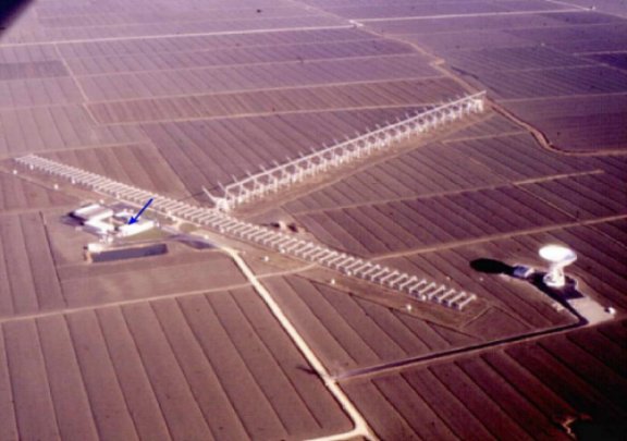
Stelio Montebugnoli is 51 years old, happily married to his Carla. He graduated from the University of Bologna as an Engineer in Electronics, and is now a Dr. Eng. in Control systems. Being in charge of Istituto di Radioastronomia (IRA) near Bologna, one of his responsibilities is to perform the upgrading of the "Northern Cross" (front page), and to manage the staff at IRA. Since he loves everything about radio, he collects old radio receivers. Other hobbies are music, especially playing the piano, and old motorbikes. Jader Monari (29) lives near Bologna, where he also attended to the University. He got his engineering degree, equivalent to MSc., three years ago in telecommunication. At IRA he is a theoretical analyst in the microwave group. Jader is also involved in SPORT - Sky Polarisation Observatory. The main goal of SPORT, is to develop a receiver for the frequency range 22 - 90 GHz. Jader is a handsome young man, and currently single. Sergio Mariotti, 34, is in his 14th year at IRA as a technician. Generally, he works with microwaves, and more specifically with the receiver of the VLBI radiotelescope (parabola with diameter = 32 m, next page). He has technical high school education, and he is very interested and skilled in instrumentation. In the spare time, he likes sport activities like bicycling, swimming and skiing. Radiotelescope station
The picture shows an aerial view of the radiotelescopes department of Istituto di Radioastronomia. The blue arrow on the picture shows where we lived.
1. INTRODUCTION1.1 Report structureIn Chapter 1, we present the background of our project, and the interested parties in the project, followed by a statement of our goals in Chapter 2. Chapter 3 contains the strategy plan for EMBLA 2000. The preparatory work for solving our problem is described in Chapter 4. Chapter 5 presents our design goals, theory, solution to the problem and results.Radioastronomy application with spectrometers is presented in Chapter 6, followed by a careful presentation of the spectrometer Sentinel II in Chapter 7. In Chapter 8, we discuss our technical solutions, results and how project challenges were solved. Finally, the conclusion summarises the outcome of our work, and how we consider our experiences from Italy.
1.2 BackgroundHessdalen, Norway, is a small valley in Holtålen situated in Sør-Trøndelag County, 30 km south-east of Trondheim. It has 170 inhabitants.Light phenomena have been observed in Hessdalen since December 1981, as big glowing balls of various shapes close to the ground. The diameter of the phenomena is from a few centimetres up to several metres. The light beams are intensive, pulsating, colour shifting and visible in a time range of a part of a second up to hours. The research on the phenomena started in 1984 by Erling Strand, Assistant Professor at Østfold College of Engineering and Natural Sciences (HiØ-IR). Scientists from all over the world have shown great interest in the Hessdalen Light Phenomena (HP), and several well-known researchers participated in an international science conference held in Hessdalen 1994. The future prospective and possibilities are great. Physicist Dr. David Fryberger (Stanford University) believes the phenomena represent a new field within science. Based on the conference-participants' discussions, this might be a new state of energy, and if we manage to capture and utilise it, a new source of energy is discovered.
1.3 CollaborationThe School of Engineering and Natural Sciences, Østfold College (HiØ-IR) plays a major role in the Hessdalen Research Project. Several student-groups have worked on, and are working on, projects aimed at establishing a professional analysis system to investigate the HP.HiØ-IR has entered into an informal collaboration with the Istituto di Radioastronomia (IRA) in Bologna, Italy. The institute collects and analyses radio-signals from space (radioastronomy). They can, with some very powerful digital spectrometers, determine the distribution of some chemical elements in the Milky Way. Because IRA has shown interest in the HP, a proposal for a 3 month joint research project between HiØ-IR and IRA in Hessdalen in the summer of 2000 has been put forward (EMBLA 2000). IRA plans to move the spectrometers Serendip IV, Sentinel I and Sentinel II to Hessdalen.
2. OBJECTIVES"The preliminary study will result in a detailed report, describing new methods of extracting measurement data from the HP through the use of techniques, equipment and algorithms from radio-astronomical research field." IRA also emphasises that the goal of the research program, EMBLA 2000, will be to investigate whether the HP occur in the radio frequency band.
Project objectives
3. SYSTEM OVERVIEW3.1 The preliminary proposalIn a preliminary document by HiØ-IR and IRA, the following proposal for Hessdalen has been put forward. They plan to install three systems located at the sites illustrated below.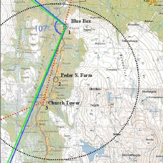
Fig. 3.1: Map of Hessdalen, with the situation of the stations.
The receiver of both sites 1 and 3 should be designed to have the front-ends, local oscillators and IF stages at the sites. The base bands are intended sent to the main control (Peder S. Farm). All the arrays will be managed from the main control room making the data collection, data storage and data post processing much more efficient. A GPS clock signal is expected to be available for instrument synchronisation. A complete Radio frequency interference (RFI) survey from 0.1 to 2 GHz (with the maximum sensitivity) is necessary, for the complete comprehension of Hessdalen RFI (Radio frequency interference) scenario. This information will be very useful for the Østfold college students visiting Medicina from April 99 onwards, in order to better design the antenna / front-end stage with the best characteristics. It will be built in the Medicina laboratories during the students' project stage, and tested in a second RFI survey (summer 1999) in Hessdalen, which will give, in the field test, a final understanding about the receiver behaviour.
3.2 The revised proposalA workshop was arranged at IRA 14.05.99. Representatives from HiØ-IR, IRA and other resource persons were present. An "updated proposal" was put forward by the staff at IRA, and the workshop participants agreed to this strategy plan.
Fig. 3.2: Updated Hessdalen stations situation. The analysis systems to be installed at the sites illustrated on previous page are described as follows.
The main control room will be at Peder S. Farm, where the overall data are received, stored and post processed.
4. BACKGROUND RESEARCH
4.1 Studying the RFI conditions in HessdalenThe analysis system which will be installed in Hessdalen, summer 2000, is of a very sensitive kind. This means that a normal environment with existing radio- and TV- channels etc could saturate the receivers, and devastate the measured signals. It is therefore necessary to find the frequency and value of these interference sources. Armed with this information, it is then possible to design filters that reject undesired frequencies.On 13th April 1999 Cecilie, Petter and our supervisor, Bjørn Gitle Hauge, left for Hessdalen. We brought instruments, tools, spare parts, cables, connectors and personal equipment. On arrival in the evening, we connected the instruments as planned, to check that the equipment was functioning. The following day, we did our research at two locations: Peder S. Farm and the Blue Box (see map in Chapter 3.2, at page 8).
4.1.1 Peder S. Farm1. Instruments:
Fig. 4.1.1: The connection for measuring the RFI conditions in Hessdalen. 2. Measuring strategy Our antenna was placed on the porch at Peder S. Farm. Before we started, we calibrated our spectrum analyzer and adjusted for the antenna factor with the amplitude correction on our analyzer. Then we followed the procedure on next page:
We repeated this procedure at vertical polarisation to see if any new frequency components had occurred. We had to do an in-depth study around 350 MHz, but found no new components. To determine true worst-case (highest level of each peak), we noted max-level bearing, and then did a close-up at each peak in this particular direction. With close-up, we mean reducing the span and raising the resolution.
The picture above is taken at Peder S. Farm, displaying Cecilie hard at work. 3. Results Figure 4.1.2, below, shows the highest level of each peak in the frequency domain. The data are collected from Appendix 4.1.
Fig. 4.1.2: RFI profile at Peder S. Farm.
4. Discussion of the results The measuring sessions went through without any particular problems. It was snowing heavily, which can cause greater free space loss (from transmitter to receiver) than usual. The receiver was, however, located not far away from our antenna, so the weather is not contributing in a big way to the measurements. To compensate for meteorological conditions and inaccurate instrumentation, 1 dB is added to the measured RFI level, and displayed in figure 4.1.2. Since our task is to suggest a receiver, fixed at 1.4 GHz, and not sweeping, these data need not be considered in our case. The data are, however, important to be taken into account in a possible sweeping receiver design.
4.1.2 Blue Box1. InstrumentsThe instruments and connections were the same as at Peder S. Farm, except we did not have the TV-monitor and the TV-receiver instrument, since the Blue Box is located in hilly terrain. 2. Measuring strategy The method was almost the same as at Peder S. Farm, but we focused more directly on the already known peaks.
3. Results The diagram below illustrates the highest level of the RFI as a function of frequency. Appendix 4.1 gave the data. The measuring is made in the bearing where the peak levels were at maximum signal level.
Fig. 4.1.3: RFI profile at Blue Box. Some screen captures from the spectrum analyzer are shown in Appendices 4.2 and 4.3. 4. Discussion of the results
The measuring at the Blue Box site was more difficult than at Peder S. Farm for practical reasons. The instruments had to be carried up the hillside, and connected in a rougher environment. However, it was not these facts that polluted our data, but a connection problem with our antenna cable. The connector was damaged, probably caused by all the turnings the antenna was put through for direction measuring. This problem occurred while examining the range from 80 - 100 MHz. 3 dB is therefore added to this range at figure 4.1.3 (and in Appendix 4.1).
When comparing the RFI of the two sites, most peaks were common. This fact makes the measuring procedure quite reliable. The conclusions about the frequencies are as follows: The RFI 952 and 468 MHz are caused by cellular phones, 182 MHz is a national broadcasting TV-channel, and the range from 87.5 - 108 MHz is occupied by several radio-channels. The staff at IRA examined these data, and they considered Hessdalen to be a "quiet" area what RFI are concerned.
5. SOLUTION TO THE PROBLEMThe design goals of the receiver are outlined in the first section. Then the superheterodyne receiver is described. In the following section, the result of the front-end measurement is presented. The next section contains the computer-simulation of the receiver, using SysCalc 3.15. In the last section the final design decision of the receiver is presented.
5.1 Design goalsThe design goals of the receiver are as follows:
5.2 The superheterodyne receiverRadiotelescope receivers are basically similar in construction to receivers used in other branches of radio science and engineering. The most common type is the superheterodyne receiver. We have selected this architecture in our receiver because of its flexibility and low cost properties. This section gives a description of this receiver's principles and functions.5.2.1 Superhet functionThe principle of the superheterodyne set, or "superhet" as it is commonly known, is to change the incoming signal. By means of "beating" it with a locally produced oscillator signal, the incoming signal changes to a lower fixed frequency. Circuits that are very insensitive to all other frequencies then amplify this lower fixed frequency, called an intermediate frequency (IF). This arrangement eventually became established as the universal approach to receiver design and remains so today.An example of the advantages of a superhet receiver can be seen when it is used to convert a signal of magnitude several GHz to a signal in the MHz region. This is primarily because low frequency components are less expensive and easier to design. The great majority of RF receivers use the superhet principle because the fixed, intermediate frequency or frequencies can lead to designs with high selectivity. Selectivity is important in the realisation of the idea of a receiver - that it should produce an output only from a true RF signal at the correct channel frequency. A superhet receiver is more selective for the same bandwidth percentage (BW %) than a direct conversion receiver. That means it has a smaller band of frequencies that it will accept, process and amplify. An example of this is as follows: Suppose you are tuned to an AM radio station at 1100 kHz. Your receiver has a BW % = 3 %. That means it will accept all frequencies from 1067 - 1133 kHz (1100 ( 3 %). If you have an interfering signal at 1130 kHz, your receiver will accept it, too. This is where a superhet receiver is useful. Without changing the BW %, the superhet receiver can reject the interference. Assume that the superhet uses a fixed IF of 455 kHz (this is commonly used for AM superhet receivers). Considering it will pass and amplify all signals in the band 455 ( 3 % = 442 - 468 kHz. When you tune the superhet receiver, you mix the incoming signal with 655 kHz (or 1555 kHz) to create the 445 kHz (centre) signal. The interfering signal will also mix with the 655 kHz and be reduced to 475 kHz, which is outside the operating band of the IF receiver and will be rejected. The superhet receiver is used in FM radios, televisions, mobile phones, satellite receivers, test equipment, etc. In many cases multiple conversion stages are required. The superhet principle can be applied in a broad frequency range (kHz - 100 GHz), and that is another reason why it is used in so many applications. A very essential component in the superhet architecture is the mixer.
5.2.2 The mixerAny non-linear device can serve as a mixer. The mixer has the function of converting the input spectrum to the first IF band, and achieves this by the use of a non-linear device(s). The mixer cannot be a linear unit, because of the Superposition Theorem for linear circuits, which states that the mixer output spectrum would be similar to the input spectrum, which is not desirable.In figure 5.2.1, we describe the functionality of an ideal mixer. It combines the incoming RF signal (from the antenna circuit) and the local oscillator (LO) signal to shift the input signal to a lower frequency. The mixer thus receives two RF signals - one at the true RF, and the other from the local oscillator.
Fig. 5.2.1: Block diagram of a RF mixer. The true input - output relationship of a mixer in the time domain can be expressed by a Taylor series:
We assume that the RF input signal to be of this kind:
Fig. 5.2.2: Second order intermodulation products, generated in the mixer. The sum and difference frequencies generated by the second power in equation (1) are called second order intermodulation products; those generated by the third power are third order intermodulation products. Usually, in receiver mixers, the sum and difference frequency output components are the only desirable ones (blue arrow, figure 5.2.2.). The sum- and difference frequencies are also known as upper and lower sideband. In order to make it clear, these sidebands are as follows: Upper sideband:
The original frequencies, their harmonics, and their sum must be removed by filtering. The filters that perform this task, and the other components in our receiver are treated in Chapter 5.6. 5.3 Omnidirectional antennaAn omnidirectional antenna is planned for the measuring station Peder S. Farm. We bought Diamond 190, a neat and self-assembled omnidirectional antenna (more information in Appendix 5.1). No datasheet was included, so we had to determine the characteristic data by doing our own measuring.5.3.1 Measuring the antennaThere are a lot of possible measurements. Measuring the gain is one of the most important, but also very difficult. To obtain accurate data, a meteorological laboratory is required. Nevertheless, we tried to find some of the characteristics during a measuring session 3rd May 1999. Another essential property of an antenna is return loss (RL).1. Instruments
Fig. 5.3.1: Gain measuring set-up. This kind of measurement requires the distance, d, between the reference antenna and the transmitting antenna, to be of a value so that the ratio of the electric field to the magnetic field is constant. We started with measuring the RL (echo). It can easily be done by considering the impedance match (ZSOURCE = ZLOAD). To measure the degree of echo, we used the network analyzer. Good match results in a low degree of echo. The RL characteristic of the antenna is shown in figure 5.3.2 and in Appendix 5.2. When measuring gain, it is necessary to have an antenna in transmitting mode. In this case we needed two different transmitting antennae, the Creative has a fmax below 1300 MHz, and the Sama has a fmax above 1300 MHz. We assembled the Diamond 190 antenna on a small wooden ladder on the roof of IRA. The transmitting antennae were located on top of a van about 100 m away, and used one at the time. All measurements were carried out in vertical polarisation. Initially we transmitted over the entire frequency spectrum from the van; to check that the system set-up was working. Then the following procedure was carried out: Creative antenna:
The RL of the antenna is characterised in the figure below.
Fig. 5.3.2: Return loss characteristic of the Diamond 190 antenna. The RL result is reliable, because the measurement was simple, and few sources of error were present (simple connection with antenna, low-attenuation cable and accurate SA). One way to determine the RL quality, is to check the amount of RL area below the 0 dB line. In our case, we have quite a large area, which indicates that the RL properties of Diamond 190 are quite good. Sergio Mariotti examined the results from the gain measuring, and they appeared to be very different. The gains for both the transmitting antennae are estimated to be 13 dB, but various values were measured. The source that polluted our data is probably reflection from trees, ground etc. From this, we learned that measuring of an antenna's gain ought to be done in a meteorological laboratory, where reflection is avoided. The gain result of the Diamond 190 antenna, could not be considered reliable, and is thus not printed in this report.
5.4 Front-endThis section discusses an amplifier's essential parameters and our measuring results. We will use it in the front of the receiver, so it is called a preamplifier (preamp). The band pass filter to be placed right after the antenna is described at the end of Chapter 5.4.5.4.1 Essential parametersWhen selecting the amplifier (amp), we especially considered three parameters: gain, noise-figure and third-order intermodulation products (IP3). These features require careful consideration in a front-end. We also had to consider availability, cost and facility of power supply.
Gain
Noise-figure (NF)
Third-order intermodulation products (IP3)
Return loss (RL) To measure it, we input a signal to a device in a given frequency range. Then the returned signal is examined. Ideally, the signal is not returned, because we want it to pass through the device, and not to return as an echo. To obtain this condition, a perfect match is required, meaning that ZSOURCE = ZLOAD. A perfect match is, in other terms equal to infinite RL. The mathematical definition is: RL = -20 log |(|, where ( is the reflection coefficient.
We selected
5.4.2 Measuring the amplifierApproachOn Monday 3rd May 1999, we carried out some practical tasks on our amp, Mini-Circuits 1217LN, with Sergio Mariotti as supervisor. He suggested we could measure the gain, return loss and IP3 properties.
Measuring gain and return loss1. InstrumentsWe used the instrument HP 8720D (50 MHz - 20 GHz), Network analyzer (NA). By using two gates, it inputs power to Gate 1, and receives power on Gate 2. From the reflected power on Gate 1 and received power on Gate 2, it can determine gain and RL. To supply the amp with 15 V, we used HP 6717A power supply.
Fig. 5.4.1: Instrument set-up for gain and return loss measuring. We tuned the frequency range for the NA to 1 - 2 GHz, and power output (Gate 1) to -30 dBm. Then we calibrated the instrument to fit our conditions. Calibration is necessary, because instruments are not intelligent. It is thus our job to give it information about our components and system. This is how the calibration was performed:
3. Results Figure 5.4.2, shows the properties of our amp. The red line is RL, green line is gain and blue line is reference level. All parameters are dB values. The marker (triangle) is set at frequency = 1.4002, displaying gain = 26.058 dB and RL = -18.763 dB.
Fig. 5.4.2: The printout from HP 8720D shows the properties of Mini-Circuits ZEL-1217LN. This laboratory session went as planned, and the NA is very accurately. We can therefore conclude that the characteristics shown in fig. 5.4.2 are reliable. When considering the RL, a rule of thumb would be: -10 dB is a poor match, -20 dB a good match, and -30 dB a superb match. Having this RL and gain, we can conclude that our amp has high quality features. The amp was a bit warm after this session done in room temperature, so a cooling device such as a little heat sink may be considered in the future work, depending on the requirements.
Measuring IP3 properties1. InstrumentsFor this session, we used the instruments described above. In addition, we employed:
Fig. 5.4.3: Set-up for IP3 measurement. Suppose we apply two close frequency peaks, f1 and f2 to a non-linear amp. It will, because of the non-linearity, generate various new frequency components (Fourier Theory). It can be shown that these components will appear as this series:
Hence, it is the two-tone, third-order that will occur in our frequency band. To see these products, it is necessary that the input signal exceed a certain level. 2. Measuring strategy To reset the NA, we turned it off. According to our lab supervisor, a freestanding instrument does not exist for such types of measuring. In order to get accurate and reliable data, the set-up has to be carefully planned, to get the best use out of the NA.
Adjustments 3. Results The figure on the next page shows the IP3 measurement result. The IP3 products are visible on each side of f1 and f2.
Fig. 5.4.4: IP3 measurement result. To calculate the IP3 properties of our amp, we used the equation: 4. Discussing of the results We calculated the IP3 properties to be 24 dB on the basis of the measuring. The manufacturer has set the IP3 to 25 dB. A measuring error of 1 dB can also in this case (with accurate instruments) be possible. The conclusion, therefore, is that the amp probably can perform within the IP3 specifications.
5.4.3 Measuring the amplifier and filterTo see how the amp and the filter work together, we had to do some measuring with both of them in the circuit. Thursday 20th May 1999, we got assistance from Alessandro Scalambra (IRA) to measure gain and RL.1. Instruments We used the NA - HP 8720D in our measuring. The amp, Mini-Circuits 1217LN and the filter, Reactel SN87-2 were connected as illustrated below.
Fig. 5.4.5: Instrument set-up for gain and return loss measuring. 2. Measuring strategy When the NA was calibrated for this kind of circuit, the measuring could start. We tuned the frequency range 0.05 GHz - 20 GHz, to see where the amp was operating. Then we used the procedure described above, in 5.4.2.
3. Results Appendix 5.5 shows the gain and RL of our amp and filter connected. The BW of the system was estimated to 1.4 - 1.26 GHz = 0.14 GHz = 140 MHz. 4. Discussion of the results As mentioned, the NA is very accurate. We can conclude that the characteristics displayed in Appendix 5.5 are reliable.
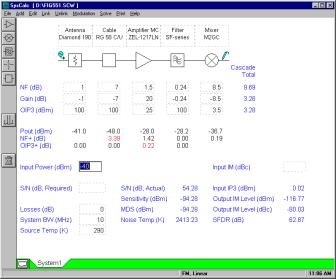
5.5 SimulationThis section describes how we simulated the receiver for the Hessdalen analysis system. The values of the first band pass- and low pass filter were qualified assumed, and the other values were taken from datasheets, or calculated with proper formulas.5.5.1 GenerallySysCalc is a Windows-based program developed by Arden Technologies, Inc. The program is for modelling noise, gain, intermodulation performance, and compression characteristics of a system of cascaded components. SysCalc's powerful features allow you to easily balance performance parameters such as dynamic range, sensitivity, spurious levels, gain distribution, temperature and tolerance variations.For an easy calculation of our front-end, we used the simulation program SysCalc, version 3.15. It could quickly help us discovering the system deficiencies with its block-to-block calculation.
Fig. 5.5.1: SysCalc's screen layout.
5.5.2 The simulationTo start the simulation we needed to design the system. We built the system by first collecting components from the toolbar. The first block on our figure (5.5.1) symbolises our antenna, Diamond 190. The second block is a generic block, which symbolises the cable, RG 58 C/U (10 m). We had to consider the cable, because it attenuates the received signal, and thereby adds noise.Our amp (Mini-Circuits ZEL-1217LN) is the third block in the system, followed by a filter, and finally a mixer. We chose a filter in the SF-series from Lark Engineering, and a mixer, M2GC from Watkins-Johnson Company, because they had suitable properties for our system. Then we entered noise-figure (NF), gain and output third order intercept point (OIP3) for these components. Most of the data were found in the datasheets, but not output intercept point. It is not always printed, it depends whether the component is active or passive. In, for example, an amp's datasheet, you may find the OIP value, but in a mixer's datasheet, only the input intercept point (IIP) is resigned. It is not difficult though, transforming it to OIP3. Output and input intercept point are related by the mixer conversion loss or gain. With that:
In our case the OIP3 for the mixer is calculated with equation 1: The mixer's NF = 8.5 [dB], and its conversion loss = -8.5. The antenna has no particularly gain, and its values are set to NF = 1, gain = -1 and OIP3 = 100. We gave also the cable and the filter OIP3 = 100, because these components are passive, and the intermodulation has therefore no meaning. On passive components the NF and gain values have the same absolute values, but with opposite signs. The filter's attenuation (Insertion loss) was calculated with this formula (3):
Hence (4): The cable attenuation can be found as a curve in the datasheet (Suhner HF-kabel / RF-cables) to be 70 dB / 100 m at the frequency, 1400 MHz. Thus a cable of 10 m will result in 7 dB attenuation (= -7 dB gain). In our case, at Peder S. Farm, the cable will be ca. 6 m, which results in 4.5 dB attenuation, and gain = -4.5 dB. The amp's specifications are obtained from its datasheet. Next step in the simulation is to determine the bandwidth (BW) and the temperature of the system. Our system has a BW = 15 MHz. The source temperature is often set to environment temperature, 290 K. In our case as well. To simulate the system, we clicked 'Solve' in the menu. The program then calculated our system's total NF, gain and OIP3, and it told us where the critical element for each parameter was. We noticed, at the Cascade Total at the System Page, that the NF was high and the gain low. To fix this, we moved the amp next to the antenna, i.e. before the cable. This gave us a considerable improvement, and we decided to place the amp near the antenna. Between the antenna and the amp, we placed a band pass filter with center frequency 1.4 GHz. Its features were qualified embraced to NF = 1, gain = -1 and OIP3 = 100, after a measuring with the amp and the filter. We also considered adding another amp, after the mixer, and we had to chose an amp with at least a range from DC to 15 MHz, since the spectrometer, SII demands BW = 15 MHz. We chose another amp from Mini-Circuits, ZHL-32A. It has a frequency range from 0.05 MHz to 130 MHz, and its features are NF = 10, gain = 25 and IP3 = 38. The datasheet follows as Appendix 5.4. The final component in the receiver, is the low pass filter, which is described in Chapter 5.6. A qualified supposition of its features are NF = 0.5, thereby gain = -0.5, and OIP3 = 100 since it is a passive component. Then we had to select the maximum input power [dBm] in order to maintain the system in the linearity region. First we chose the sensitivity value where the S/N ratio is zero [dB]. The sensitivity is the minimum input level necessary to detect a signal. That means the input signal whose power level is equal to the equivalent noise power present at the system input. The input noise power is determined by the systems bandwidth, source temperature and effective system noise temperature, i.e.
When setting the input power equal to the sensitivity, the IP3 products are below the noise threshold. Then increasing the signal in (Pin), the intermodulation products will be higher than the threshold, and the back-end will detect these as incoming signals. This is not a preferred situation. Therefore the next step, would be to find the input power, from testing several values, such that the Output IM Level are equal to the Pout value from the first input power selection. This will give the maximum Pin we can use for our system, Pin = -33.7 dBm. If we insert a value higher than this one, the Pout may not be correct, because the non-linearity of the system generates intermodulation products above the noise threshold. The figure below shows our simulated receiver suggestion
Fig. 5.5.2: Our receiver's properties.
5.6 The proposed receiverAfter well-considered work with lots of alternatives and simulations, our suggestion for a low cost receiver for the Hessdalen analysis system is shown in figure 5.6.1. We have not been able to build the system, since the delivery time is long for some of the components. The decision whether we will buy all these components also needs careful discussion with the staff at HiØ-IR. The receiver is however simulated with SysCalc as described in the previous chapter.
Fig. 5.6.1: Suggestion for a receiver for the Hessdalen analysis system.
The antenna
Band pass filter I To replace this filter after EMBLA 2000 expires, we may order a band pass filter with centre frequency at 1.4 GHz and about 200 MHz bandwidth. It does not need a very steep characteristic, so the insertion loss and price may be low. We suggest, for example, a filter from the SF-series (Lark Engineering), at US $ 500 (price source: IRA).
The preamplifier
Cable
Band pass filter II
The mixer
Synthetizer
Amplifier
Filter
Back-end
GPS reference clock
Total cost To estimate the total cost for a front-end, receiver and back-end system, we have to add the synthetizer and GPS clock expenses. Synthetizer price is US $ 5000, and the GPS clock solution is estimated to about US $ 100. In total the system amounts to about US $ 6500. The Hewlett Packard synthetizer is an expensive module, but also a very useful instrument, and absolutely necessary to obtain the stability a back-end requires. In addition, it can be used in many other exercises. If HiØ-IR do not have the opportunity to buy such an instrument before the summer 2000, IRA will supply it for the 3 months while the research program proceeds.
6. BACK-END
6.1 Serendip IVSerendip IV (SIV) is a high-resolution spectrum analyzer, developed by UC Berkeley. It is used as a surveillance system, able to detect narrow-band terrestrial radio frequency interference (RFI) and signals that might come from planets like Earth. This last discipline is known as SETI (Search for Extra-Terrestrial Intelligence).One SIV crate features 32 million channels in a 19.2 MHz range, giving a very high resolution. To cover a wider frequency span, it is possible to connect several SIV crates in parallel. The data from the Arecibo dish antenna in Puerto Rico (diameter = 320 m), is, for instance, connected to 5 SIV crates. "Piggy-back" modeThis expression is often mentioned in SIV contexts. It means that the SIV system works in parallel with the ongoing observation, reducing costs. It is possible to have 1 - 8 boards in the SIV crate (Fig. 6.1.1, next page).A top-down approach of SIV is shown in fig.6.1.1.
Fig. 6.1.1: Software algorithms make it possible to display the detected frequencies as spots in a two-dimensional matrix. With a sweeping receiver as in this example, it is possible to scan a wide frequency range. The total sweeping time (fmin - fmax) will then be a multiple of 1.68 seconds. In some situations, it is more convenient to have the receiver centred to a fixed frequency with 19.2 MHz total bandwidth. The advantage with such a property is a total processing time of 1.68 sec per spectrum. This feature is a good approach to detect (fast) frequency variation (Doppler shift). A practical display example of figure 6.1.1 is shown in fig 6.1.2.
Fig. 6.1.2: The SIV frequency-time chart. This mode makes it is easier to discover regular RFI patterns (compared to figure 6.5.1). The vertical lines on the figure illustrate terrestrial RFI.
6.2 Sentinel ISentinel I (SI) is a spectrometer like SIV, developed by the staff at IRA. The difference between SIV and SI is the resolution and the total bandwidth. SI is a low-resolution spectrometer with 10 kHz binwidth, and 10 MHz bandwidth. An M62 board equipped with the Ultra Fast C62 DSP from Texas Instruments performs the FFT. A schematic diagram of the system is shown in figure 6.2.
Fig. 6.2: Sentinel I architecture.
6.3 Sentinel IISentinel II (SII) is a medium resolution spectrometer, also designed by IRA. Bandwidth is 15 MHz with a programmable number of channels from 1k up to 8k. In this system, a double Xeon, Pentium Processor performs FFT. The schematics is shown below:
Fig. 6.3: Sentinel II architecture.
6.4 Post processingFrom the receiver, we acquire a measured signal as function of time. We want to examine which frequency components this signal consists of. To determine this, Fast Fourier Transform (FFT) is applied.
Fig. 6.4.1: Digital data is acquired from the radiotelescope-receiver, and transformed from time to frequency domain by Fast Fourier Transform. The result of the FFT can be displayed as a frequency spectrum. The figure below may give you an intuitive understanding of what Fourier Transform really performs. The difference between Fourier Transform and FFT is of course that FFT is faster. What makes it possible to do it fast, are single passes, known as Butterfly.
Fig. 6.4.2: The time and frequency coherence can be estimated with Fourier Transformation.
6.5 Sentinel I & II visualisation software
Fig. 6.5.1: Sentinel I visualisation in "Spectrum mode" (one-dimensional) with omnidirectional antenna. Please note that it is possible to choose only some of the antennae if desired. From figure 6.5.1, it is clear that the transfer function of the front-end is shaping the displayed signal. It can be removed by clicking view mode "Normaliz". A flattened curve will then be displayed. This software is also capable of presenting the signal in "Serendip" mode (frequency-time) if you choose 'Serendip'. An example is illustrated below.
Fig. 6.5.2: "Serendip mode" with omnidirectional antenna. The vertical perforated stripe is a regular RFI signal. It is possible to display signals from antennae with different bearings, as well as from an omnidirectional. A SIV visualisation of directive antennae is shown at figure 6.5.3.
Fig. 6.5.3: "Serendip mode" with multiple directional antennae (each covering 45 degrees). Please note that in this case, the same signal is fed to all antennae for testing. In this example, the N-W and South antennae are inactivated. The last two display modes require a fixed frequency band. In the following, we will explain some of the features at the "options-panel".
FFT channelsWhen choosing the number of FFT channels, we decide the frequency resolution of the spectrometer. Note that increased frequency resolution (more channels) means decreased time resolution. Suppose we want to improve our frequency resolution with a factor of 2. Then our time resolution aggravates equally. This is because more channels mean higher acquisition time, since we have to acquire a double number of points.FFT Burst SizeThe burst size tells us how many times the signal is averaged per display. When averaging the signal, the level of a regular RFI signal will be its mean, and equivalent for the noise. The noise is, however random in its nature (Gaussian distributed), and thus the mean of such a signal decreases proportional with (the square root of) the burst size number. In this way, it is possible to discover a regular RFI signal embedded in noise. An example of this may be figure 6.5.2, where the number of averages is high (32). In this case, tuning down the burst size (for instance 2 averages) resulted in an invisible regular RFI signal.The disadvantage with increasing the burst size is a higher processing time (computing averages takes time). ThresholdWith the threshold, it is possible to "cut-away" frequencies, at a level that is lower than a certain value. The benefit of this, is the opportunity to remove noise and reduce the points to be stored on our disk. By doing this, we might remove an interesting, weak signal, though. Thus, the Threshold limit should be tuned to match the signal we to examine.BandwidthAs an option, the total reviewed bandwidth is tuneable. For instance, if the bandwidth of the signal examined is known, we can tune our BW to adapt to this, and obtain optimal channel resolution.7. FUTURE WORK7.1 The planAt the work-shop arranged at IRA 14th May, some future aspects of EMBLA 2000 were discussed. Those present agreed to attempt to involve more scientists from different disciplines, and perhaps apply more instruments. This strategy aims to improve the research approach and increase the probability of revealing the physical explanation behind the light phenomena.The researchers planned another more formal meeting before next summer, and also to further discuss the most efficient approach for EMBLA 2000. IRA recommends another stay for Cecilie and Petter at the institute, in order to build and characterize our simulated receiver. 7.2 What now?In our project, we have acquired and characterised a front-end, suggested a design for a high quality receiver and described applied radioastronomy methods. What now?We have been working towards EMBLA 2000 and designed a receiver by using simulation facilities. To set up the spectrometer Sentinel II (SII), it is necessary to realise our suggested receiver, or possibly discuss other receivers. SII is planned to be employed in Hessdalen during EMBLA 2000, and also to be connected to HiØ-IR's radiotelescope. In the following, a comprehensive figure and various examples of SII applications are displayed. Sentinel II low cost spectrometer ~ US $ 5000
Fig. 7.2.1: A rough schematic of Sentinel II. The Sentinel II is a good investment at US $ 5000, compared to Serendip IV (SIV), costing about US $ 50.000. The SIV system has, however, a higher resolution. It is not possible to compare them directly, because they have different fields of application. SIV is most efficient at detecting weak narrow band signals, while SII would be a better approach to detect signals of a wider span. The SII can be employed in many different applications, some of them illustrated in the following pages. Sentinel II applications1. Back-end for the Østfold College 4 m dish antenna, searching for H-lines in the Milky Way. Some chemical elements such as, for example, formaldehyde, water, methanol etc can be determined by frequency analysis on the Sentinel display.
Fig. 7.2.2: Sentinel II applied in Hydrogen search. 2. Meteor detection
Fig. 7.2.3: Detecting meteors. It is possible to detect meteors with the SII system. The meteor can be discovered at the output file as a skew dotted line, like this:
3. Geophysical resource exploration Characterisation of geological substrata by analysing the echo from many small explosions performs underground analysis.
Fig. 7.2.5: Geophysical resource exploration. 4. RFI monitoring Radio band(s) occupation control
Fig. 7.2.6: Surveillance of RFI conditions. 5. Natural phenomena study in the VLF field (lightning, noise etc)
Fig. 7.2.7: Studying very low frequencies. Example of applications to RFI monitoring and band occupation control:
Fig. 7.2.8: Data are integrated and presented in the "3D visualisation mode", making it possible to get an overview of the RFI scenario at a location. As can be seen from the figures above, a lot of applications are possible. Sentinel II can work as an extremely powerful spectrum analyzer, available to present the result in several ways. The presentation mode can be adapted to the kind of measuring / analysis we want to perform.
8. DISCUSSION8.1 Technical discussionFront-endOur front-end, consisting of antenna, filter and preamplifier, is of good quality. The problem with an omnidirectional antenna is, however, that it acquires a lot of noise from the ground. This is not a big problem though, because it can be replaced with a different antenna if so is desired. The most important consideration regarding the front-end in our case, is the noise property. Our front-end is designed to have sufficiently low noise figures, providing the necessary conditions in the first stage of our receiver.
Receiver
Spectrometer
8.2 General discussionWhat is special about our final year project is that we stayed abroad for half our project period. It is no doubt a challenge to work in another language than Norwegian, especially as we have no previous knowledge of Italian. Thus we communicated in English with the staff at IRA. The people at the institute were very conscious about speaking slowly to make a point. This approach made us able to communicate both ways, having only minor, insignificant misunderstandings.The internal communication between the two of us, worked out fine, since we argued for our own points of view rather than quarrelled. We thought it was an advantage, sharing a project between only two persons, because less adjustments to each other is required. It is also easier to control the written material (report writing), when only two persons are involved. From our point of view, there are some factors critical for succeeding in a study project abroad. Showing decency and openness is a necessary human feature. A certain amount of language knowledge and the ability to use Internet as a tool, certainly will not hurt either. The most important factor, as we see it, is to achieve communication. For us, this part is an extremely important supplement to the technical skills.
8.3 Our stay at IRAThe radiotelescope station of IRA is situated on the countryside, 20 km east of Bologna. Thus the surroundings were calm, making it possible to get our work done. We were accommodated in one apartment each, giving us some privacy when desired. In order to obtain sufficient study facilities, IRA had prepared a study room at arrival. A Pentium PC, connected to Internet and the "network neighbourhood" was to our disposal. In this way, any desired software was provided, as well as images and documents from IRA's large file library.The staff at the institute is highly skilled in radioastronomy and electronics, but also willing to teach and help us with any problems or technical matters, despite their tight time schedule. Moreover, any request was carefully taken care of to ensure that both our project and stay could be a pleasant experience.
9. CONCLUSIONA front-end with antenna, filter and amplifier is acquired and characterised. It will be implemented as first module in our receiver suggestion. We have, by data simulation, designed a medium sensitive, low cost receiver of high quality. From IRA's experience, this simulation program matches the reality surprisingly well. We can thus conclude that our design process has been sufficient to design a reliable receiver. The spectrometer Sentinel II has been presented in several interesting physical experiments, and can be considered a versatile, efficient frequency instrument. IRA (and we) would strongly recommend it for the EMBLA 2000 program, and as a spectrometer connected to the HiØ-IR radiotelescope. One of the objectives with a final year project is to develop communication skills. It is our opinion that a student project abroad, succeeds even more in this than a final year project "at home". Taking this in account, and all our interesting experiences and friendships made, it is easy to recommend a study project abroad. In total, this lead us to conclude that we have achieved our goals. But without great help from the staff at IRA, we could not have succeeded in the same way.
Appendix 5.1Datasheet: Diamond 190
Omnidirectional antenna
Self-assembled
Appendix 5.2Return loss characteristic of the Diamond 190 antenna
Appendix 5.5Filter and preamplifier in serial connection
Abbreviations (alphabetical)
ReferencesBibliography:
| |||||||||||||||||||||||||||||||||||||||||||||||||||||||||||||||||||||||||||||||||||||||||||||||||||||||||||||||||